Tinkering and Benchmarking SeaweedFS
⚠️ This article is an automated translation. While I personally reviewed the content before publication, some inaccuracies may remain. Read the original French version.
During this year, I was faced with a client with the thorny issue of object storage in business: Within this company, it is impossible to consider a “cloud” solution for their storage: indeed, they have many regulatory and legal constraints that formally prevent them from delegating data storage to an external service provider. The question therefore arises: how to provide them with effective, scalable, on-premise object storage, and preferably without paying absurd license fees.
If our gaze had initially turned to MinIO, it was without counting on the absolutely catastrophic management by the eponymous company of its community version: end of distribution of builds, withdrawal of several important features… And that’s how my gaze turned to SeaweedFS, a project I’ve been following from afar for a (very) long time, but that I had never had time to experiment with in extreme conditions.
Today, then, we are testing SeaweedFS to store data in active-active replication across several datacenters, in real-time. Just that.
SeaweedFS, its Life, its Work
Created in 2014, SeaweedFS is an open-source distributed file system, designed to efficiently store and access billions of files. Its main strength lies in its file access time in O(1); in other words: no matter the size of your cluster, the file access time will be the same. Built to work in single-node, multi-node, single-datacenter, multi-datacenter, Seaweed positions itself as a Swiss Army knife of storage, ready to meet any need. Furthermore, some features of Seaweed are rare enough to highlight, notably the presence of erasure coding and a POSIX-Compliant FUSE (tl;dr: you can mount your object storage like a USB key on your PC or server).
Of course, Seaweed comes with a whole range of connectors: S3, Kubernetes CSI, etc. In short, on paper, it’s the perfect product for storage; all the more reason to make me want to try it!
A few terms of art before we continue together:
- SeaweedFS works with master nodes responsible for maintaining consistency and knowledge of the cluster;
- Then, SeaweedFS needs volume nodes, which store the data.
- Finally, SeaweedFS has filer, an additional server that allows exposing volumes through multiple “classic” interfaces for storage: FUSE, WebDAV, S3, etc.
SeaweedFS offers real-time replication on the cluster. For this, we use a three-digit code to define replication, XYZ, where:
Xindicates the number of times the data must be replicated in other datacenters;Yindicates the number of times the data must be replicated in the same datacenter but in a different rack;Zindicates the number of times the data must be replicated in the same rack.
Thus, a replication at 200 indicates that the data must be replicated in 2 other datacenters than the original one (we therefore store the data 3 times). A replication at 101 indicates that we will store the data in a second datacenter, and a second time in the original rack.
When registering a volume node, we will therefore inform its datacenter and its rack. Attention, SeaweedFS is consistency-first: Data writing is only confirmed when all requested replicas have been written!
Today’s experiments do not focus on security considerations: Seaweed offers several options to control access to data, so we do not explore this part since the solution is available “out of the box”.
Tests Performed (multi-DC without internal network)
Mission Objectives
The objective of this test is to verify the behavior of a SeaweedFS cluster in active-active multi-master replication on the S3 storage and FUSE (Seaweed Filer) part: performance, error rate, replication, scalability, resilience, backup, and restoration.
The observed elements will be:
- Seaweed availability: is the cluster capable of responding to our requests?
- Data availability: Am I able to access 100% of my data?
- Performance: What are the write and random read throughputs, both in S3 and FUSE mode?
Installation
For this full-scale experimentation, we will provision 7 VMs from several different providers:
- Volume nodes:
- 2x EM-A116X-SSD (Scaleway - Dedibox Elastic Metal - Aluminium Range) (€0.077/h)
- 2x CAX21 (Hetzner - Cloud - Shared Cost-Optimized) + 400GB block storage (total cost: €0.09/h)
- Master + filer nodes:
- 2x CX23 (Hetzner - Cloud - Shared Cost-Optimized) (€0.0067/h)
- 1x DEV1-M (Scaleway - Cloud - Development Instances) (€0.0198/h)
Important considerations:
- Seaweed will be installed directly on the machines. The target OS is Debian 13 (trixie).
- For cost reasons, deployment will be fully automated (Ansible playbooks and OpenTofu are available on GitHub)
- Once again, security is not the priority of our experiment: we will be in “open bar” mode (all flows open).
- To simplify our task, we will create DNS records (the domain is at OVH):
master-X.lab.forestier.refor master nodes;volume-X.lab.forestier.refor volume nodes;masters.lab.forestier.re(DNS round-robin on master nodes);volumes.lab.forestier.re(DNS round-robin on volume nodes).
All the data allowing to deploy our test infra is available on GitHub.
⚠️ Important Considerations
It is imperative to note that the deployment conditions of the solution are extremely poor: We are on 2 providers without dark / dedicated fiber available, so we transit through the public Internet network (with the induced latency and hops); on heterogeneous hardware that is not intended for “production-grade” storage. The performance obtained is therefore to be put into perspective, taking into account these technical specificities. In an optimal world, we would be in 2 datacenters on equivalent hardware, with a dedicated fiber allowing to transit directly and at high speed.
Details and Performance of the Base Infra
For the test below, we are therefore on 2 different datacenters, without a dedicated network for communication between these two datacenters. Here is the traceroute DC2 (Hetzner) -> DC1 (Scaleway). The average ping latency is 40ms, and the average transfer rate is 48Mbps (obtained by downloading a 1GB file).
traceroute to 2001:bc8:711:756:dc00:ff:fed1:3f71 (2001:bc8:711:756:dc00:ff:fed1:3f71), 30 hops max, 80 byte packets
 1  fe80::1%eth0 (fe80::1%eth0)  2.936 ms  3.123 ms  3.217 ms
 2  31801.your-cloud.host (2a01:4f9:0:c001::2827)  0.426 ms  0.446 ms  0.470 ms
 3  * * *
 4  spine3.cloud1.hel1.hetzner.com (2a01:4f9:0:c001::a0e9)  1.370 ms spine4.cloud1.hel1.hetzner.com (2a01:4f9:0:c001::a0ed)  1.522 ms  1.783 ms
 5  * * *
 6  core32.hel1.hetzner.com (2a01:4f8:0:3::6bd)  1.136 ms core31.hel1.hetzner.com (2a01:4f8:0:3::6b9)  0.758 ms core32.hel1.hetzner.com (2a01:4f8:0:3::6bd)  0.708 ms
 7  * * *
 8  * * *
 9  core2.ams.hetzner.com (2a01:4f8:0:3::201)  27.276 ms core2.ams.hetzner.com (2a01:4f8:0:3::205)  27.136 ms core2.ams.hetzner.com (2a01:4f8:0:3::201)  27.192 ms
10  2a01:4f8:0:e0f0::11e (2a01:4f8:0:e0f0::11e)  28.698 ms  27.542 ms  27.525 ms
11  2001:bc8:1400:2::3e (2001:bc8:1400:2::3e)  28.857 ms 2001:bc8:1400:2::18 (2001:bc8:1400:2::18)  28.909 ms 2001:bc8:1400:2::42 (2001:bc8:1400:2::42)  28.841 ms
12  2001:bc8:0:1::18f (2001:bc8:0:1::18f)  37.518 ms 2001:bc8:0:1::18b (2001:bc8:0:1::18b)  37.905 ms 2001:bc8:0:1::18f (2001:bc8:0:1::18f)  37.231 ms
13  2001:bc8:400::36 (2001:bc8:400::36)  38.773 ms  38.391 ms  38.242 ms
14  2001:bc8:400:1::1b1 (2001:bc8:400:1::1b1)  38.988 ms  38.634 ms 2001:bc8:400:1::1bb (2001:bc8:400:1::1bb)  38.377 ms
15  2001:bc8:410:1018::1 (2001:bc8:410:1018::1)  41.636 ms  41.872 ms  40.920 ms
16  2001:bc8:410:1018::c (2001:bc8:410:1018::c)  36.908 ms  37.206 ms  37.860 ms
17  3f71-fed1-ff-dc00-756-711-bc8-2001.instances.scw.cloud (2001:bc8:711:756:dc00:ff:fed1:3f71)  36.878 ms  36.993 ms  37.837 ms
The cluster is configured so that all volumes and buckets are in replication 100: Once in another datacenter. All files are therefore committed by Seaweed between DC1 and DC2.
Disk performance is (obtained via dd of a 10GB file):
- On DC1 storage nodes: Write 2.6GBps / Read 4.9GBps
- On DC2 storage nodes: Write 304MBps / Read 323MBps
Smoke Test - Verify the Cluster is UP
After launching the installation script, we access the three administration panels (port 23646/tcp). The graphical interface is in alpha, so small bugs are visible; notably on the “Master nodes” part, which only indicates the node currently elected by Raft (the others are hidden). However, the cluster logs clearly indicate that the cluster is in HA with an active quorum.
The volumes are all visible and correctly labeled. We are ready to start!
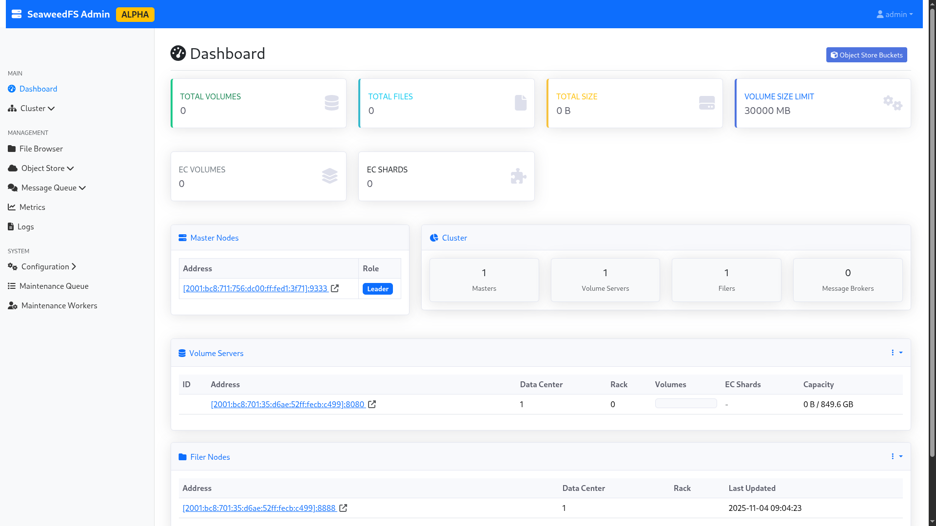
Figure 1: The SeaweedFS admin interface.
Loss of a Master Node (No Load)
First of all, you should know that SeaweedFS is based on the Raft consensus algorithm, widely used in the world of highly available systems: Docker Swarm, Kubernetes, MariaDB and many others use this consensus protocol. Generally speaking, it is considered that to survive the loss of n nodes, you need 2n+1 nodes within your cluster. For example, a cluster composed of 3 masters can continue to function with 1 missing node, a cluster of 5 with 2 nodes, etc. In Raft, the controllers elect a “leader”, who is responsible for actively managing the cluster; while the others content themselves with maintaining the quorum. When this node is lost, a new election takes place to define a new leader.
Upon loss of a master node, the cluster manages to find itself and come back online. Two scenarios:
- If the lost node is not the main node: The remaining nodes (including the leader) notice the loss of the node and continue to function without it. The operation is transparent.
- If the lost node is the main node: The remaining nodes launch an election to obtain a new leader. In the tested cases, the cluster takes a few seconds (4-5 seconds) to find a consensus, during which the cluster is no longer manageable. However, already created volumes continue to function.
Note: SeaweedFS does not necessarily recommend having several masters: according to them, this only meets rare scenarios and introduces additional load to cluster management. The authors take Google as an example, which has been running single-master on its home storage solution for years. Although I subscribe to the idea that making management highly available meets a rather infrequent need, I can attest (having lived and experienced it) that these kinds of systems have already saved me on several occasions.
Performance in Object HTTP (S3) Mode in Nominal Configuration
For this example, I will build two buckets from the Seaweed graphical interface, without quota, and send several GB of random data to each bucket. The first bucket will be filled by a third-party server at OVH already in my possession, the other with my personal PC. I use the rclone tool to connect to the buckets.
In more detail, I will simulate sending all the source code of OpenBAO (https://github.com/openbao/openbao) from my PC: about 350MB, spread over more than 5000 files. All over an unstable 4G connection.
On my server, I will simulate sending 2GB of random data broken down into 1MB files. The server has an unmetered 1Gbps fiber optic. Two radically different use cases.
My rclone has the default configuration of the S3 provider: maximum 4 parallel uploads; no optimization on TCP connection preservation or anything. To make matters worse, I’m going to pass through the DNS round-robin, which will therefore make my rclone change host at each file upload. In a real world, we would have a network device type F5/HAProxy that would give us a beautiful VIP with anti-affinity.
The rclone configuration is as follows:
- Type: S3
- Provider: SeaweedFS
- AccessKey / SecretKey: Those generated for my user in the GUI
- Endpoint: http://volumes.lab.forestier.re:8333/
- ACL: Private
The test starts at 10:44:00. Very quickly, the SeaweedFS graphical interface starts showing the files being populated. During the whole time of the test, the graphical interface remains accessible, and I can instantly re-download a file already uploaded from the UI. The wait is imperceptible on that side.
I cut the test at 10:54:00. The two rclone had time to send:
- For the one on unstable 4G: 2.1MB in 456 objects (i.e., 3.5kb/s)
- For the one on fiber: 408MB in 408 files (i.e., 680kb/s)
The performance is… Abominable; probably because of my DNS round-robin. So I slightly change the configuration of my rclone: I point one rclone to http://volume-1.lab.forestier.re:8333/, the other to http://volume-3.lab.forestier.re:8333/ (I selected these nodes at random).
I launch at 10:57:10, and cut at 11:07:10. To compare, I created two additional buckets that served me to launch this version of the configuration. The results are as follows:
- For the one on unstable 4G: 2.2MB in 368 objects (i.e., 3.6kb/s);
- For the one on fiber: 376MB in 376 objects (i.e., 626kb/s).
Contrary to my intuition, forcing a specific filer attenuates performance. I modify my rclone once more to increase the number of files to send in parallel (and put back my DNS round-robin), since my dataset lends itself to it: many small files. I set the value to 20; and I relaunch at 11:10:30. At 11:20:30, the results are as follows:
- For the one on unstable 4G: 2.2MB in 368 objects (i.e., 3.6kb/s);
- For the one on fiber: 376MB in 376 objects (i.e., 626kb/s).
Obviously, a performance glass ceiling applies to our infrastructure; probably because of inter-datacenter communication. Following these more than doubtful results, I decided to modify my test scheme (we’ll talk about it in a few seconds).
Despite disappointing performance, it is still worth noting that:
- The files are all well replicated on disk between the two datacenters, as requested;
- The graphical interface and the APIs exposed by Seaweed held up perfectly against the demand;
- The interconnection with rclone is validated.
Tests Performed (multi-DC with internal network)
In order to continue my tests in better conditions, I decided to change my approach and abandon the idea of operating on two different providers: I will deploy all of my test infra at Scaleway, on 2 datacenters belonging to them, with a virtual private network (VPC) to connect my services between the two DCs.
This approach will allow me to experiment with my storage system in conditions a bit closer to reality: a single internal network, reduced hops, improved connectivity.
Here is the new lab:
- Volume nodes:
- 4x EM-A116X-SSD (Scaleway - Dedibox Elastic Metal - Aluminium Range) (€0.077/h)
- Master + filer nodes:
- 3x DEV1-M (Scaleway - Cloud - Development Instances) (€0.0198/h)
All on a VPC. The nodes will therefore communicate with each other via the internal VPC IP, and will no longer make the big internet loop.
It is worth noting that I made sure to preserve the previous proportions, to avoid biasing the test. Finally, for information, I kept Scaleway simply because disk performance was higher than on Hetzner’s servers. This is quite logical, since the machines I use at Scaleway are dedicated servers billed hourly, while at Hetzner, they are instances with a network mount point (which inevitably degrades performance). It is therefore a purely technical choice related to the purpose of the project; Hetzner’s solutions being, on a daily basis, as pleasant to use as Scaleway’s (and that’s a very nice compliment, Scaleway being my favorite cloud provider!).
The servers will be deployed on Scaleway’s WAW-2 and WAW-3 zones.
For information, here is the performance obtained with this setup:
- Ping WAW-2 => WAW-3: 1.96ms (and via public link: 2.22ms)
- Transfer WAW-2 => WAW-3: 267Mbps (and via public link: 34Mbps)
- Disk writing: exactly the same as before.
We’re off for another round! And to do things properly, we start over… with the same operating procedure.
As for earlier, the installation scripts are available on GitHub.
Performance in Object HTTP (S3) Mode in Nominal Configuration
We resume the same operating procedure as the previous test (OpenBAO, rclone, etc.). The results obtained in 10min00s of upload are:
- For the one on unstable 4G: 2.2MB in 392 objects (i.e., 3.75kb/s);
- For the one on fiber: 408MB in 408 objects (i.e., 696kb/s).
Obviously, performance plateaus even with a much faster infra between the nodes. Two test ideas then come to me:
- Try with large files (50MB), to check the impact of repeated opening/closing of TCP streams;
- Try with volumes without replication.
With Larger Files
For practical reasons, I only launch from my fiber-connected PC, with 50MB files instead of 1MB. After only 6min54s, the 5GB of files (100 chunks of 50MB) are online… i.e., 12.36MB/s, a much more honorable result.
Important note: I kept the upload of OpenBAO source code from my unstable 4G in the background, to maintain similar cluster usage.
The S3 protocol therefore seems to support large files much better (which is not surprising: large files require fewer TCP connection opens/closes, so less time lost waiting for a reconnection to the server).
For conscience’s sake, I decided to keep my test without replication, but I decided to add, out of curiosity, the “without replication AND with large files” test.
Interestingly, the bucket appears with a size of 10.1GB in the interface (because replicas are counted in the actual size of the bucket).
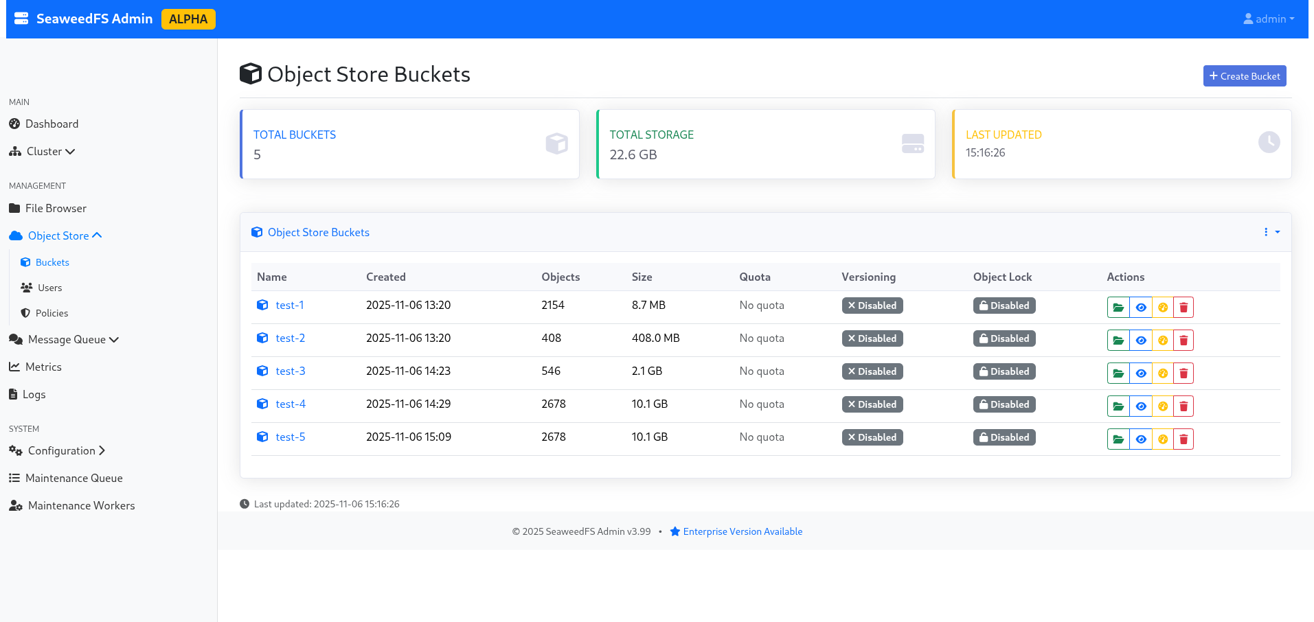
Figure 2: The list of buckets, indicating 10.1GB due to replication.
I take advantage of the reconfiguration time to explore the admin interface a bit, and notably the “volumes” part, which allows me to see the actual split of my data, their replication, their status, which node is active and which is in replication… In short, it’s quite neat as a technology, and even for a storage noob like me, it’s understandable!
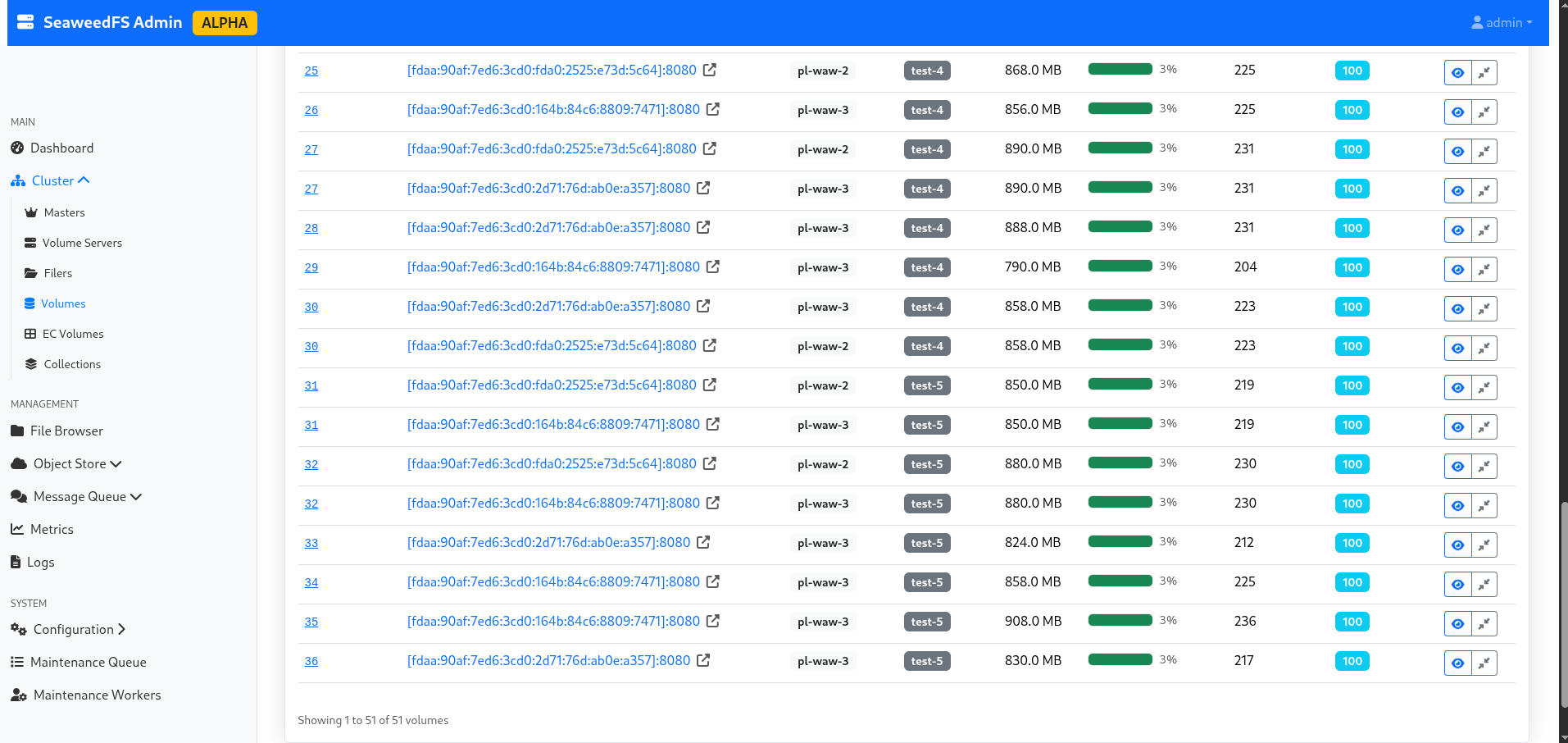
Figure 3: List of volumes per bucket.
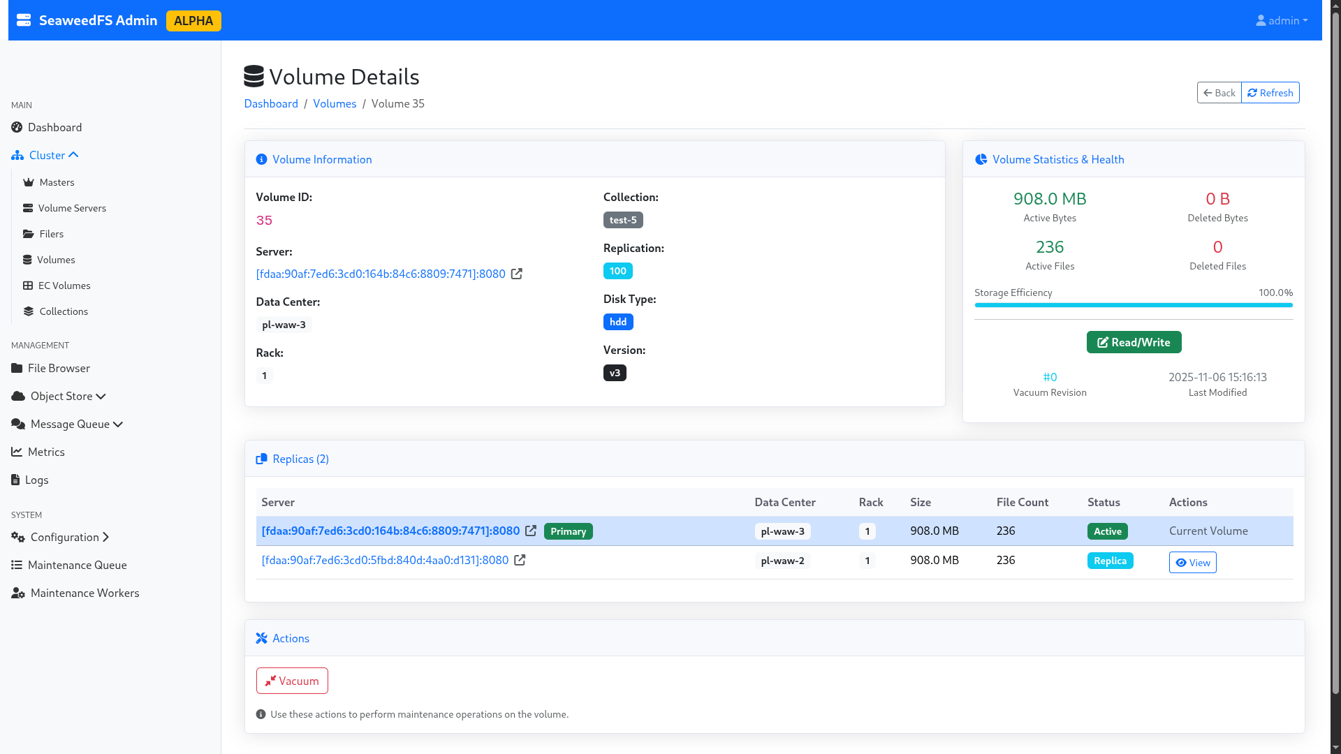
Figure 4: Details of a volume.
Without Replication and with Large Files
I relaunch my send of 5GB of 50MB files, still with my OpenBAO source code send in the background (the thread of this blog post, in the end!).
The upload takes a total of 6min16s without replication, i.e., a throughput of 13.61MB/s. A slight improvement, but nothing to jump for joy about. However, interestingly, this means that replication seems to happen at a very low cost in terms of performance loss.
For fun, I play a bit: I try to send a single large 1GB file without replication, then with replication. The time it took:
- Without replication: 35 seconds (i.e., 29.25MB/s)
- With replication: 35 seconds (i.e., 29.25MB/s)
=> Replication therefore has no significant impact on performance in single-write (and on multi-write, negligible as we were able to see before).
It is also worth noting that 29.25MB/s gives ~234Mbps. However, the WAW-2 => WAW-3 link is advertised at 267Mbps. It is therefore highly likely that the network is once again acting as a bottleneck in our test. Having no other infrastructure capable of doing better, I will be content with this result. However, if someone has a dedicated backbone between two geographically distant datacenters with 1Gbps and NVMe type disks, I’m interested in the feedback!
Performance in Object HTTP Mode with Outage Simulations (master/storage/datacenter)
For this little experiment, I’m going to send 5GB of random files of 50MB each again, and, during the transfer, I’m going to perform a kill -9 on a random volume node. The goal is to see the cluster’s behavior, and look at the impact on performance. I’ll be in replication 100 (i.e., real-time replication across the 2 datacenters). Then, I’ll do the same experiment with a kill -9 on a random master node. Finally, I’ll do this action on an entire datacenter!
So let’s go for the first step.
Loss of a Storage Node
I start my experiment at 16:51:00, and I cut the server volume-pl-waw-2-0 at 16:51:11, right in the middle of an rclone transfer. By “cut”, I mean by that that I cut not only the volume node, but also the filer node, to simulate real node downtime. The write operation finishes at 16:57:23, i.e., 6min12s (13.76MB/s). As a reminder, without node loss, we were at 6min54s (12.36MB/s).
Even if the throughput is higher with one less node, the improvement is to be put into perspective: we are at less than 10% difference, with many factors coming into play, notably the quality and availability of the network between the upload server and the cluster. The difference is therefore not significant.
I take the opportunity to verify the data availability in the current case, by downloading the entire test-5 bucket, which was in active replication and heavily used the deleted server. I manage to download all the data without problem, the cluster having detected the node loss.
⚠️ Important Limitation: SeaweedFS does not have auto-heal in the community version; the cluster therefore does not rebalance data automatically to other nodes to fill the void. On a purely personal basis, having experienced auto-rebalances with CephFS, I almost consider this an advantage… But everyone has their opinion. 😉
I relaunch the volume and filer on the disconnected server, to return to nominal configuration. The node automatically comes back up in the pool, and Seaweed starts using it again, as if nothing had happened.
Loss of a Master Node
Here we go again, and this time, my victim will be lab-master-1. I start the copy at 17:07:10, and I cut the node at 17:07:39. The rclone continues to run without error. The graphical interface continues to expose itself. The copy finishes in 6min34s… i.e., no visible impact.
I turn the node back on and continue my tests.
Loss of a Datacenter
As a reminder, our infra is deployed across two regions: “WAW-2” and “WAW-3”. The goal here is to completely cut “WAW-2” in the messiest way possible (kill -9 of everything containing weed in the name), to simulate a sudden and unexpected failure of an entire datacenter.
I start the copy at 17:29:30, and I simultaneously cut the entire “WAW-2” region (1 master, 2 volumes) at 17:29:45. The rclone quickly starts displaying 500 errors, as writing can no longer be performed because the entire “WAW-2” datacenter is offline; and SeaweedFS waits for all requested writes to be validated to confirm writing a file. So I relaunch the “WAW-2” datacenter to return to a nominal case.
	status code: 500, request id: 1762447203809093757, host id:
2025/11/06 16:40:05 ERROR : chunk_0012.bin: Failed to copy: InternalError: We encountered an internal error, please try again.
The user-side error message.
In a few seconds, the cluster comes back to life, and the transfer resumes. It should be noted that during the loss of the “WAW-2” datacenter, the data remained perfectly accessible in read-only mode. However, we have a “hard-limit” of the model here: SeaweedFS prioritizing consistency over availability, the latter interrupts any write action if the cluster is no longer in a state to validate all desired writes. However, we have two workaround solutions, which we are going to mention: temporary replication change, and multi-cluster asynchronous replication.
Note: A “rich man’s” option would be to have a third datacenter available, and keep a 100 replication. Thus, if one datacenter falls, it is still possible to redundant the data as requested. However, this option has limits, the first being that in a business, one doesn’t grow a datacenter out of the ground that easily…
Temporary Replication Change
The idea of this solution is to temporarily change the replication configured on the cluster, in order to allow users to write again. This operation requires restarting the master nodes still alive (fortunately, one can do it one after the other, and therefore not bring down the entire cluster). In order to preserve a minimum of redundancy, one can play on our replication to ask Seaweed to replicate at a minimum in another rack; for example by going from a 100 to 010 replication. Let’s experiment with this possibility.
As a trial, I drop “WAW-2” again, and I try to modify the replication to “001”: this allows asking the two remaining servers on “WAW-3” to synchronize between themselves on the same rack (to keep resilience), and no longer wait for the other datacenter. On the 2 volume servers, I modify the defaultReplication to 001, and I relaunch the nodes 1 by 1 (to avoid a full-downtime).
My 5GB of data (100 * 50MB) then writes in 4min04s, without any rclone error!
I then turn the “WAW-2” nodes back on. Listing the volumes, I can see volume “77”, which corresponds to my experiment, which has a 001 replication. However, now that my second datacenter is available again, I want to replicate my data on it!

Figure 5: Replication in 001 mode, which is not our usual target at all.
For this, SeaweedFS will allow us to modify, directly in command line, the volume replication, and force the “rebalance” of the cluster. Warning, during this operation, the volume will switch to read-only! It is therefore essential to warn your users of such an operation.
In order to give our affected volume the right value back, I launch a weed shell. I start with a lock, in order to get the lock and avoid another user launching administration actions during my tasks.
Then, I launch volume.configure.replication -volumeId 77 -replication 100, in order to modify the replication of my currently created volume.
Finally, volume.fix.replication -force allows launching the rebalance. Be careful not to forget the -force, otherwise SeaweedFS will only do a dry-run! Once the operation is finished, I remember to unlock.
> lock
> volume.configure.replication -volumeId 77 -replication 100
> volume.fix.replication -force
volume 77 replication 100, but under replicated +2
replicating volume 77 100 from [fdaa:90af:7ed6:3cd0:164b:84c6:8809:7471]:8080 to dataNode [fdaa:90af:7ed6:3cd0:5fbd:840d:4aa0:d131]:8080 ...
volume 77 processed 130.00 MiB bytes
volume 77 replication 100 is not well placed [fdaa:90af:7ed6:3cd0:164b:84c6:8809:7471]:8080
deleting volume 77 from [fdaa:90af:7ed6:3cd0:164b:84c6:8809:7471]:8080 ...
volume 77 [fdaa:90af:7ed6:3cd0:164b:84c6:8809:7471]:8080 has 40 entries, [fdaa:90af:7ed6:3cd0:2d71:76d:ab0e:a357]:8080 missed 0 and partially deleted 0 entries
volume 77 [fdaa:90af:7ed6:3cd0:164b:84c6:8809:7471]:8080 has 40 entries, [fdaa:90af:7ed6:3cd0:5fbd:840d:4aa0:d131]:8080 missed 0 and partially deleted 0 entries
> unlock
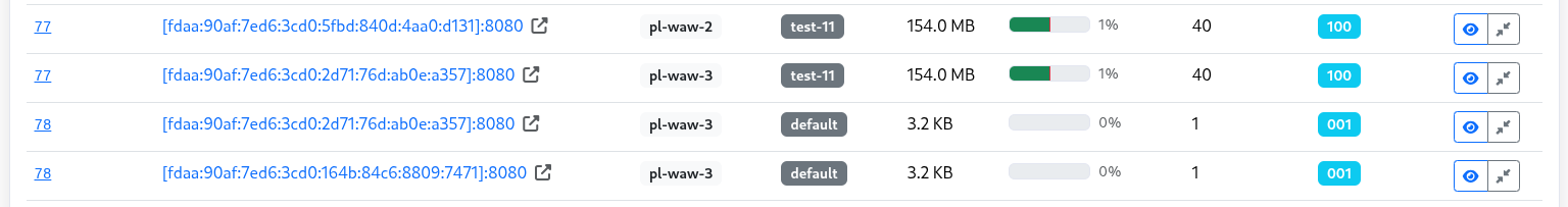
Figure 6: Our volume is back in 100 replication hurray!
This approach allows keeping a certain flexibility in data management, while continuing to provide service during the failure. The disadvantage is having to modify the replication manually, but objectively, are you ready for that when you lose an entire datacenter?
Multi-DC Asynchronous Replication
Another option would be to completely change the deployment philosophy, so as not to have a single cluster over two datacenters, but two clusters; one per datacenter. This philosophy is presented in the SeaweedFS documentation, and has the advantage of performing asynchronous synchronization between datacenters.
However, this means giving up the guarantee of consistency in favor of availability. This is an approach worth considering depending on your needs. In the case I wanted to test, the lack of data consistency was not acceptable; so I didn’t push this option further.
Performance in FUSE and WebDAV Mode
For this test, we are going to resume our cluster in “nominal” mode (cross-datacenter replication) on WAW-2 and WAW-3. I follow the documentation indicated on the SeaweedFS wiki (FUSE, WebDAV).
The client will be my PC, connected to a 2.5Gbps fiber. The disk is an NVMe (Phison Electronics Corporation PS5021-E21 PCIe4). The write speed is 2.4GBps, and the read speed is 4.2GBps.
We are going to calculate the time to write 1GB of random data in 1MB, 50MB blocks, and the time required to retrieve them. I will also perform the test with random data in 4kb blocks, but with fewer files (to avoid it taking me all day).
FUSE Mount
To start a FUSE mount, just run on your machine ./weed mount -filer=volumes.lab.forestier.re:8888 -dir=fuse/ -filer.path=/fuse-test -volumeServerAccess=filerProxy. This command will mount the /fuse-test folder of the SeaweedFS cluster into ./fuse/ on your computer.
From there, I create 3 folders from my terminal: 4kb, 1MB and 50MB, to store the corresponding files. Then, with date and cp, I copy the previously generated files, and I retrieve the execution times:
(Note: I strongly suspect my NVMe disk of being limiting in the 4kb and 1MB tests.)
- 4kb (22528kb in 5399 files):
- Write: 16min13s (973s); i.e., 23.15kb/s
- Read: 4min25 (265s); i.e., 85.01kb/s
- 1MB (1048612kb in 1024 files):
- Write: 3min54s (234s); i.e., 4481kb/s (4.37MB/s)
- Read: 1min12s (72s); i.e., 14564kb/s (14.22MB/s)
- 50MB (1075204kb in 20 files):
- Write: 28s; i.e., 38400kb/s (37MB/s)
- Read: 46s; i.e., 23374kb/s (22.82MB/s)
- Copy of OpenBAO GitHub repository (372480kb in 6063 files):
- Write: 17min49s (1069s); i.e., 348kb/s
- Read: 5min12s (312s); i.e., 1193kb/s (1.16MB/s)
We notice that performance in FUSE is much higher than in S3 mode! I am almost frustrated with the 50MB test, because I think I am limited by the server’s public bandwidth (as a reminder, we estimated it at 45MB/s a bit earlier). Given that my test takes place the next day, we are in a probable margin of error.
Furthermore, I must say that I am quite surprised by these performances: Google Cloud Platform’s FUSE mount is about 10 times less fast, and supports about 10 times fewer features: we must salute the fundamental work done by SeaweedFS developers, who offer a totally POSIX-compliant FUSE, with support for symlinks and other joys; where even the hyperscalers have not yet ventured. In short, it’s solid!
WebDAV Mount
My filer being already configured to expose a WebDAV endpoint, I just need to mount it with davfs2: sudo mount.davfs http://volumes.lab.forestier.re:7333/dav /mnt/dav, and I relaunch the same experimental protocol (important note: WebDAV writing is asynchronous; I therefore take into account the time until the last write operation is validated):
- 4kb (4928kb in 1000 files):
- Write: 5m23s (323s); i.e., 15.25kb/s
- Read: 1m32s (92s); i.e., 52.56kb/s
- 1MB (1048612kb in 1024 files):
- Write: 5m25s (325s); i.e., 3226kb/s (3.15MB/s)
- Read: 3min21s (201s); i.e., 5216kb/s (5.09MB/s)
- 50MB (1075204kb in 20 files):
- Write: 1m07s (67s); i.e., 16047kb/s (15.67MB/s)
- Read: 46s; i.e., 23374kb/s (22.82MB/s)
As can be seen, WebDAV is systematically slower than the FUSE mount; so might as well stick with FUSE.
Stress Test
Now that we have played with SeaweedFS, it’s time to get serious! We are going to instantiate 10 DEV1-S instances at Scaleway, directly connected to our previously created VPC. I also modify the filer configuration to now listen on the internal VPC IP. You understood, the goal is to look at the performance of our system in conditions as close to real as possible: our SeaweedFS clients are now on the same network as our storage array, this looks like a real business network, where VMs are on the same network as storage arrays.
In order to preserve realistic network isolation, I only expose the filer nodes to my instances, which act as intermediaries to the volume servers.
On each machine, I create 1024 files of 1MB (so 1GB of data, i.e., 1048616kb), and 41 files of 50MB (so 2050MB of data, i.e., 2099212kb). I then mount on each machine a FUSE mount, each to a separate bucket (to simulate real-world usage conditions, where each VM stores its own data, in a bucket isolated from others).
Before launching my simultaneous copy, I launch it on a single node, to have a point of comparison with the FUSE mount previously performed on my computer. Here are the results:
- 1MB (1048616kb in 1024 files):
- Write: 1m02 (62s); i.e., 16913kb/s (16.51MB/s)
- Read: 19s; i.e., 55190kb/s (53.89MB/s)
- 50MB (2099212kb in 41 files):
- Write: 43s; i.e., 48818kb/s (47.67MB/s)
- Read: 33s; i.e., 63612kb/s (62.12MB/s)
The difference is incredible! On 1MB files, the order is 4x; and on 50MB, the order is 2x. Performances are much more acceptable and consistent with what can be expected from such a system.
Now, it’s time for the stress-test. Each node will send its 3GB of data, and retrieve them, and this 6 times (so 3 * 10 * 6 = 180GB of data). I put in the table above the time of the first write/read cycle per machine, and the last.
| Machine | stress-0 | stress-1 | stress-2 | stress-3 | stress-4 | stress-5 | stress-6 | stress-7 | stress-8 | stress-9 |
|---|---|---|---|---|---|---|---|---|---|---|
| First execution - Write | 2min09s | 2min23s | 2min36s | 3min22s | 3min39s | 3min48s | 5min04s | 5min03s | 4min45s | 5min17s |
| First execution - Read | 3min52s | 3min24s | 3min24s | 3min18s | 3min03s | 3min04s | 2min08s | 1min49s | 2min11s | 1min31s |
| Last execution - Write | 2min35s | 2min42s | 3min47s | 2min40s | 2min51s | 2min57s | 3min39s | 4min29s | 3min59s | 4min03s |
| Last execution - Read | 1min39s | 1min32s | 1min53s | 2min20s | 4min03s | 3min48 | 3min40s | 3min07s | 3min27s | 3min12s |
Or, in kb/s equivalent (based on a total of 3147828kb):
| Machine | stress-0 | stress-1 | stress-2 | stress-3 | stress-4 | stress-5 | stress-6 | stress-7 | stress-8 | stress-9 |
|---|---|---|---|---|---|---|---|---|---|---|
| First execution - Write | 24401kb/s i.e. 23.82MB/s |
22012kb/s i.e. 21.49MB/s |
20178kb/s i.e. 19.70MB/s |
15583kb/s i.e. 15.21MB/s |
14373kb/s i.e. 14.03MB/s |
15133kb/s i.e. 14.77MB/s |
10354kb/s i.e. 10.11MB/s |
10388kb/s i.e. 10.14MB/s |
11045kb/s i.e. 10.78MB/s |
9930kb/s i.e. 9.69MB/s |
| First execution - Read | 13568kb/s i.e. 13.25MB/s |
15430kb/s i.e. 15.06MB/s |
15430kb/s i.e. 15.06MB/s |
15898kb/s i.e. 15.52MB/s |
17201kb/s i.e. 16.79MB/s |
17107kb/s i.e. 16.70MB/s |
24592kb/s i.e. 24.01MB/s |
28879kb/s i.e. 28.20MB/s |
24029kb/s i.e. 23.46MB/s |
34591kb/s i.e. 33.78MB/s |
| Last execution - Write | 20308kb/s i.e. 19.83MB/s |
19431kb/s i.e. 18.97MB/s |
19673kb/s i.e. 19.21MB/s |
19673kb/s i.e. 19.21MB/s |
18408kb/s i.e. 17.97MB/s |
17784kb/s i.e. 17.36MB/s |
14373kb/s i.e. 14.03MB/s |
11701kb/s i.e. 11.42MB/s |
13170kb/s i.e. 12.86MB/s |
12954kb/s i.e. 12.65MB/s |
| Last execution - Read | 31796kb/s i.e. 31.05MB/s |
34215kb/s i.e. 33.41MB/s |
26904kb/s i.e. 26.27MB/s |
22484kb/s i.e. 21.95MB/s |
12954kb/s i.e. 12.65MB/s |
13806kb/s i.e. 13.48MB/s |
14308kb/s i.e. 13.97MB/s |
16833kb/s i.e. 16.43MB/s |
15206kb/s i.e. 14.84MB/s |
16394kb/s i.e. 16.01MB/s |
We notice that in general, we have maximum and minimum performance on each segment that can go from single to double: this is explained because the machines at the very beginning or very end are privileged, since their processes start a few seconds before/after everyone else. Here are the gaps noted:
- First write: min. 9.69MB/s, max. 23.82MB/s
- First read: min. 13.25MB/s, max. 33.78MB/s
- Last write: min. 11.42MB/s, max. 19.83MB/s
- Last read: min. 12.65MB/s, max. 33.41MB/s
The notion of read/write time in O(1) seems to be confirmed: the gap between the performance of the first and last read/write is not significant.
It is also worth noting that we are probably reaching a limit of the Scaleway server SSDs here (which are, as a reminder, servers at 7 cents an hour, nothing to be ashamed of then). Indeed, during the write/read period, the machines never reached their CPU/RAM limits: Peaks at 25% CPU were observed on the storage nodes; the masters remained impassive. I put below captures of peak write usage (on the last execution), and 5 seconds after the last read.
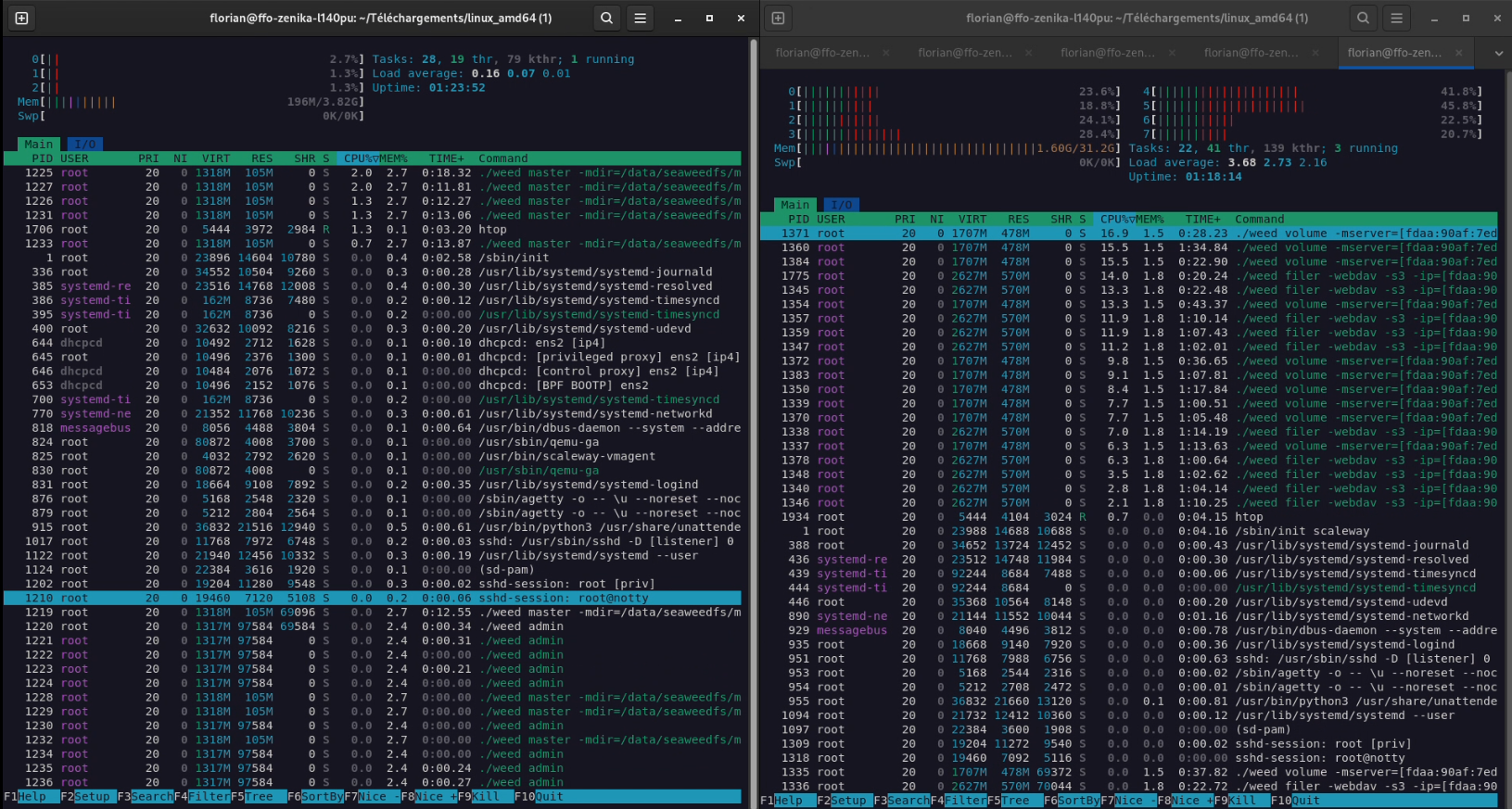
Figure 7: Cluster load in full write. Left, the master node currently “leader”; right, a storage node.
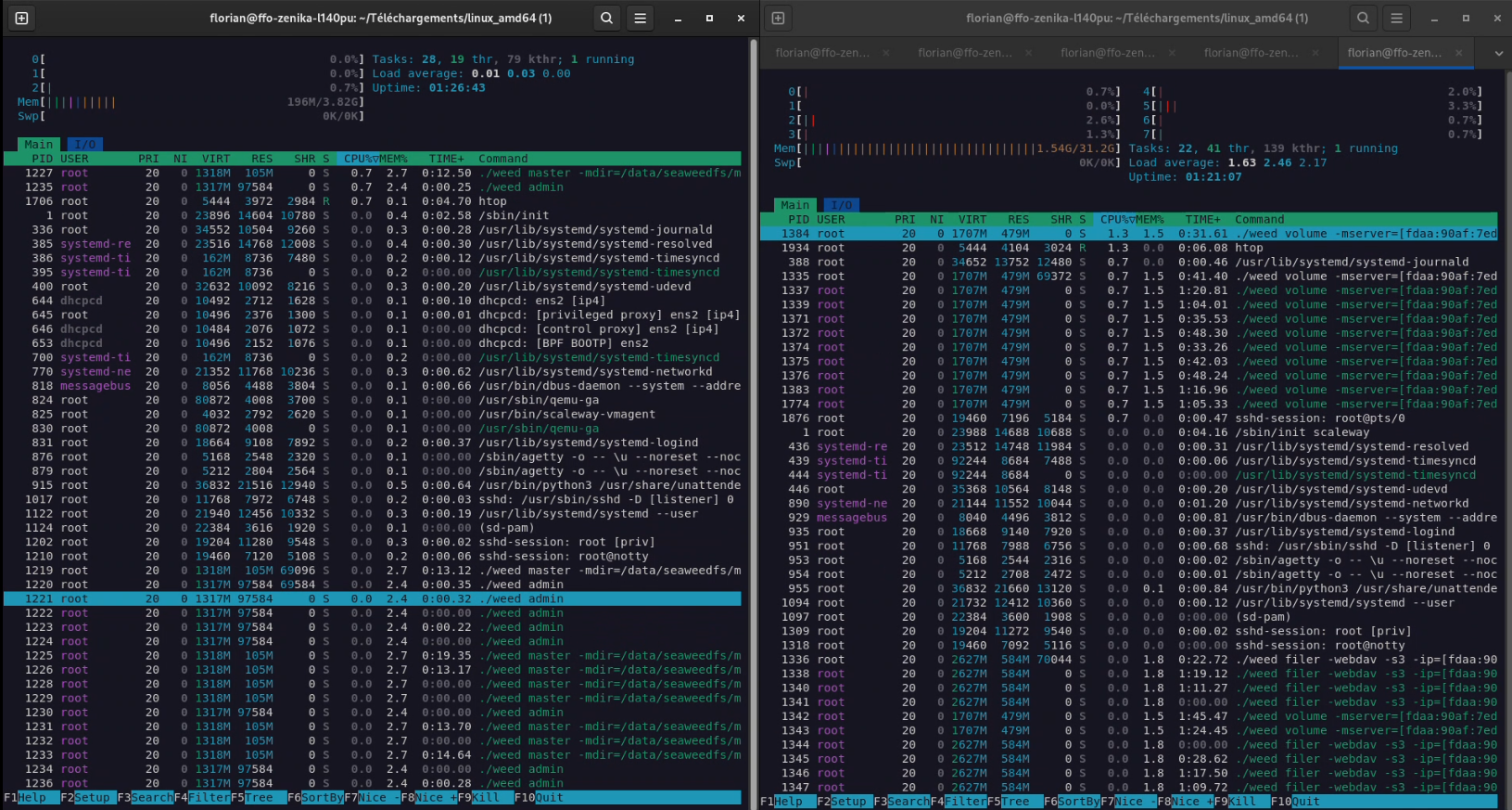
Figure 8: Cluster load 5s after the last read. Left, the master node currently “leader”; right, a storage node.
In any case, the stress-test passed with flying colors: the cluster easily handles 180GB of ingested data in just 20 minutes, with 10 clients simultaneously connected performing very intensive actions.
Interconnectivity with Kubernetes (CSI)
As a reminder, our initial need was to provide storage arrays for enterprise applications. And today, business applications are mostly deployed on Kubernetes. So I decided to try interconnecting our SeaweedFS with a Kubernetes cluster. For this, I used a small K3s cluster (1 master, 2 workers) that I had at my disposal.
I followed the documentation available on the SeaweedFS wiki (CSI). The installation is done with a simple Helm chart.
Once the driver is installed, I created a StorageClass pointing to our filer (via its internal VPC IP).
apiVersion: storage.k8s.io/v1
kind: StorageClass
metadata:
  name: seaweedfs-storage
provisioner: seaweedfs-csi-driver
parameters:
  filer: "10.0.1.1:8888" # Internal VPC IP of one of our filers
Then, I created a PersistentVolumeClaim (PVC) using this StorageClass.
apiVersion: v1
kind: PersistentVolumeClaim
metadata:
  name: seaweedfs-pvc
spec:
  accessModes:
    - ReadWriteMany
  storageClassName: seaweedfs-storage
  resources:
    requests:
      storage: 5Gi
And finally, I created a Pod using this PVC.
apiVersion: v1
kind: Pod
metadata:
  name: seaweedfs-pod
spec:
  containers:
    - name: seaweedfs-container
      image: nginx
      volumeMounts:
        - name: seaweedfs-volume
          mountPath: /usr/share/nginx/html
  volumes:
    - name: seaweedfs-volume
      persistentVolumeClaim:
        claimName: seaweedfs-pvc
Everything worked perfectly! The PVC was correctly created on SeaweedFS (it appears as a folder in the filer), and the Pod was able to mount it and write to it.
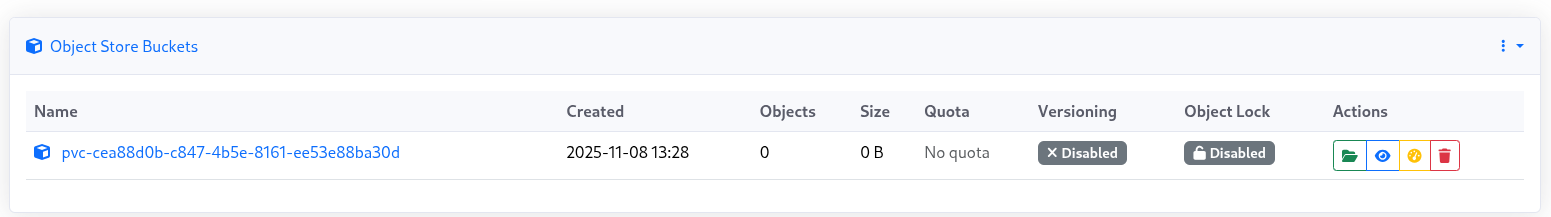
Figure 9: The PVC correctly created on SeaweedFS.
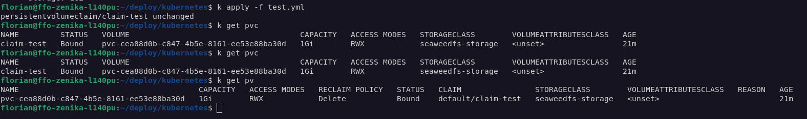
Figure 10: Details of the mount in the container.
The CSI of SeaweedFS also supports ReadWriteMany (RWX) mode, which allows several Pods to access the same volume simultaneously. This is an extremely practical feature for some business applications (like CMS, for example).
Conclusion
SeaweedFS is a very pleasant surprise. If its name can make one smile (it translates to “seaweed” in French), its features and performance are very serious.
Its strong points are:
- Simplicity: deployment is very fast, and the architecture is easy to understand.
- Performance: file access in
O(1)is not a myth, and the FUSE mount is one of the best I’ve tested. - Flexibility: Seaweed adapts to many use cases (S3, FUSE, WebDAV, Kube CSI).
- Resilience: multi-master and real-time replication are solid features.
However, there are still some points to improve:
- Documentation: sometimes a bit light or scattered on the wiki.
- Graphical Interface: still in alpha, with some bugs and lack of some features.
- Auto-heal: missing in the community version (must be done manually via weed shell).
In conclusion, SeaweedFS is an excellent alternative to MinIO or Ceph for companies that want to keep control of their data on-premise, without paying exorbitant license fees and with high performance. It’s a project to follow closely!
Bonus
For those who want to see the cluster in action during the stress-test, here is a small video of the monitoring (Grafana).